Introduction to Dynamic Programming
Have you ever written a recursive solution that looked completely correct, and ran fine on small inputs, but crashed the moment you gave it a slightly larger input as a result of the poor computer running out of memory on the call stack or timed out?
If you have, there’s a good chance you’d just met a problem with overlapping subproblems - and the fix for it is one of the most important tools in a software engineer’s toolbox: Dynamic Programming (DP).
The Motivation
Let’s start with a classic example: computing the n’th Fibonacci number.
long long fibonacci(int n) {
    if (n < 2) return n;
    return fibonacci(n - 1) + fibonacci(n - 2);
}
This looks clean, it looks correct, and for small n it works perfectly fine. But try calling fibonacci(45) and watch your program grind to a halt. Why? Because this recursive solution makes roughly 2^n function calls - (Where is the 2 coming from? Note the 2 recursive function calls of fibonacci(n - 1) and fibonacci(n - 2) within fibonacci(n)). Therefore, fibonacci(45) alone triggers over a billion calls to compute a result that could have been computed in 45 simple steps.
The root cause becomes obvious if you draw out the recursion tree: fibonacci(5) calls fibonacci(4) and fibonacci(3). But fibonacci(4) also calls fibonacci(3). Both of those calls eventually call fibonacci(2), fibonacci(1), and fibonacci(0) - over, and over, and over again. We are re-solving the exact same subproblems thousands of times, throwing away the answer each time, only to recompute it moments later. That is pretty wasteful right?
This is precisely the kind of wasteful repetition that Dynamic Programming exists to eliminate.
What is Dynamic Programming?
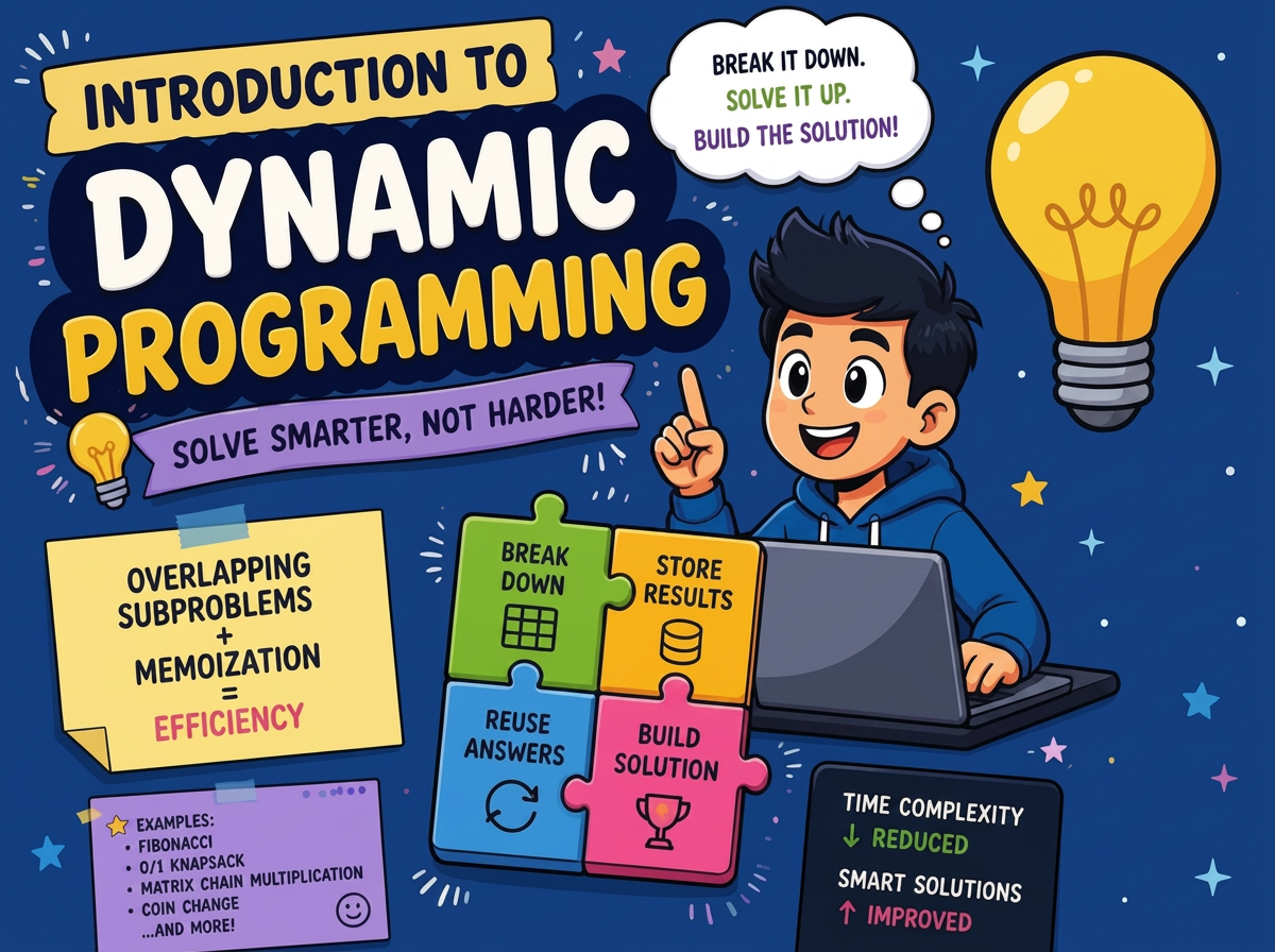
Dynamic Programming is an algorithmic technique for solving problems by breaking them down into smaller subproblems, solving each subproblem only once, and storing (or “caching”) its result so it never has to be recomputed. Instead of solving the same subproblem repeatedly, we solve it once and simply look up the answer whenever we need it again.
A problem is a good candidate for DP when it exhibits two key properties:
- Optimal substructure - the optimal solution to the overall problem can be constructed from optimal solutions to its subproblems.
- Overlapping subproblems - the same subproblems are encountered again and again while solving the larger problem.
If both properties hold, DP can typically take an algorithm from exponential time down to polynomial time :often linear or quadratic. That is a significant improvement of the performance which your clients would be super happy to hear!
Two Ways to Apply DP
There are two standard techniques for implementing a DP solution:
- Top-down (Memoization) - Keep the natural recursive structure of the problem, but store the result of each subproblem the first time it’s computed. On subsequent calls with the same input, simply return the stored result instead of recomputing it. I have discussed a similar technique in my previous post about python’s lru cache.
- Bottom-up (Tabulation) - Flip the approach entirely: start from the smallest subproblems (the base cases) and iteratively build up to the final answer, storing each intermediate result in a table (usually an array or a 2D grid) along the way. Both techniques solve every subproblem exactly once. The difference is direction - top-down starts from the original problem and recurses “down” toward the base cases, while bottom-up starts at the base cases and works “up” toward the original problem.
Let’s apply both techniques to our Fibonacci example.
1. Top-down: Memoization
#include <vector>

long long fibonacciMemo(int n, std::vector<long long>& memo) {
    if (n < 2) return n;
    if (memo[n] != -1) return memo[n]; // Already computed - return cached result

    memo[n] = fibonacciMemo(n - 1, memo) + fibonacciMemo(n - 2, memo); // Note the recursion we still we have here
    return memo[n];
}

long long fibonacci(int n) {
    std::vector<long long> memo(n + 1, -1); // -1 means "not computed yet"
    return fibonacciMemo(n, memo);
}
The recursive structure is identical to our original naive solution. The only change is the memo vector, which remembers results we’ve already computed. Now fibonacci(45) makes only 46 unique calculations instead of over a billion.
2. Bottom-up: Tabulation (no recursions!)
#include <vector>

long long fibonacci(int n) {
    if (n < 2) return n;

    std::vector<long long> dp(n + 1); // This is the table mentioned before which is 1-D in this case.

    //A very important feature: start the base cases
    dp[0] = 0;
    dp[1] = 1;

    for (int i = 2; i <= n; ++i) {
        dp[i] = dp[i - 1] + dp[i - 2]; // Build the answer from previously computed values
    }

    return dp[n];
}
Here, there is no recursion at all. We start at the base cases dp[0], dp[1] and iteratively fill the table left to right, with each entry depending only on the entries that came before it. By the time we reach dp[n], we have our answer!
Both versions run in O(n) time and O(n) space - a massive improvement over the original O(2^n) recursive solution!!
What Makes a Problem a DP Problem?
Not every problem benefits from Dynamic Programming, and it’s important to recognize the difference. Here are the telltale signs that a problem is a good DP candidate:
- The problem asks for an optimum, a count, or a possibility - phrases like “find the minimum/maximum,” “count the number of ways,” or “is it possible to” are common DP signals - I am going to discuss some common example below.
- The problem can be broken into smaller subproblems of the same type - the solution to the problem for input
ndepends on solutions for smaller inputs liken-1,n-2, and so on. - The naive recursive solution recomputes the same subproblems - if you can draw a recursion tree and see repeated branches, that’s overlapping subproblems in action.
- Decisions made now affect future options - many DP problems involve a sequence of choices (include/exclude, take/skip) where each choice narrows down what’s available for the remaining problem.
DP is usually not the right tool when:
- There are no overlapping subproblems. Problems like merge sort or binary search split into genuinely independent subproblems that never repeat - that’s plain divide and conquer and not DP.
- A greedy choice is always locally and globally optimal. Problems like the classic “activity selection” or Huffman coding can be solved with a simple greedy strategy, without needing to explore or cache all subproblem combinations.
- There is no optimal substructure. If the best solution to the whole problem cannot be constructed from the best solutions to its parts, DP will not help.
With that in mind, let’s have a look at some example Dynamic Programming problems.
1D DP Example: Climbing Stairs
Problem: You are climbing a staircase with n steps. Each time, you can climb either 1 or 2 steps. In how many distinct ways can you reach the top?
The naive recursive approach
At any given step, you either got there by taking 1 step from n-1, or by taking 2 steps from n-2. So the total number of ways to reach step n is the sum of the ways to reach n-1 and n-2.
int climbStairsNaive(int n) {
    if (n <= 2) return n;
    return climbStairsNaive(n - 1) + climbStairsNaive(n - 2);
}
This should look familiar - it’s structurally identical to our Fibonacci problem, and it suffers from the exact same overlapping subproblems issue.
The DP approach (bottom-up)
#include <vector>

int climbStairs(int n) {
    if (n <= 2) return n;

    std::vector<int> dp(n + 1);
    dp[1] = 1;
    dp[2] = 2;

    for (int i = 3; i <= n; ++i) {
        dp[i] = dp[i - 1] + dp[i - 2]; // Ways to reach step i = ways to reach (i-1) + ways to reach (i-2)
    }

    return dp[n];
}
This runs in O(n) time instead of exponential time, and it demonstrates a common DP pattern: each state depends only on the previous one or two states.
1D DP Example: House Robber
Problem: You are a robber planning to rob houses along a street. Each house has some amount of money, given in an array nums. You cannot rob two adjacent houses (doing so triggers an alarm). What is the maximum amount of money you can rob without alerting the police?
This problem introduces a new wrinkle: at each house, you must make a decision - rob it, or skip it - and that decision affects what you can do next.
Defining the recurrence
In any DP problem, it is crucial to first identify the recurrence of the problem.
Ex:-
For house i, you have two choices:
- Skip house
i- your total is whatever you could rob up to housei-1. - Rob house
i- your total isnums[i]plus whatever you could rob up to housei-2(since you cannot rob both the housesiandi-1).
You have to take the better of the two options: dp[i] = max(dp[i-1], dp[i-2] + nums[i]).
#include <vector>
#include <algorithm>

int rob(std::vector<int>& nums) {
    int n = nums.size();
    if (n == 0) return 0;
    if (n == 1) return nums[0];

    std::vector<int> dp(n);
    dp[0] = nums[0];
    dp[1] = std::max(nums[0], nums[1]);

    for (int i = 2; i < n; ++i) {
        dp[i] = std::max(dp[i - 1], dp[i - 2] + nums[i]); // Best of skipping vs robbing house i
    }

    return dp[n - 1]; // final result is at the end of the dp vector.
}
Notice the pattern: we’re no longer just accumulating a running total - we’re actively choosing between alternatives at every step, and the DP table stores the best decision made so far. This “choice-based” recurrence is one of the most common shapes you’ll see in DP problems, including the 2D examples coming up next.
2D DP Example: 0/1 Knapsack
Problem: Given n items, each with a weight and a value, and a knapsack with a maximum weight capacity W, find the maximum total value you can carry without exceeding the capacity. Each item can either be included whole or left out entirely - you cannot take a fraction of an item (hence “0/1”).
This is where DP grows from a single dimension into two: our state now needs to track both which item we’re considering and how much capacity remains.
As an example, let’s say we have an array of values each associated with a weight as shown below. Lets assume the maximum capacity of the knapsack is 10. Our problem is to find the maximum total value we can take from this.
| Index: | 0 | 1 | 2 | 3 | 4 |
|---|---|---|---|---|---|
| Value: | 5 |
4 |
2 |
7 |
3 |
| Weight: | 4 |
1 |
3 |
2 |
5 |
Defining the recurrence
Let dp[i][w] represent the maximum value achievable using the first i items with a weight capacity of w. For each item i, we again have two choices:
- Exclude item i - the best value is whatever we could achieve using the first
i-1items with the same capacityw:dp[i-1][w]. - Include item i (only possible if
weight[i] <= w) - the best value isvalue[i]plus the best we could achieve with the firsti-1items and the remaining capacityw - weight[i]. We take the better of the two:dp[i][w] = max(dp[i-1][w], value[i] + dp[i-1][w - weight[i]]).
#include <vector>
#include <algorithm>

int knapsack(std::vector<int>& weights, std::vector<int>& values, int W) {
    int n = weights.size();
    std::vector<std::vector<int>> dp(n + 1, std::vector<int>(W + 1, 0));

    for (int i = 1; i <= n; ++i) {
        for (int w = 0; w <= W; ++w) {
            // Option 1: exclude item i-1 (0-indexed array, so item i is weights[i-1])
            dp[i][w] = dp[i - 1][w];

            // Option 2: include item i-1, if it fits
            if (weights[i - 1] <= w) {
                dp[i][w] = std::max(dp[i][w], values[i - 1] + dp[i - 1][w - weights[i - 1]]);
            }
        }
    }

    return dp[n][W];
}
Here, dp is a 2D grid, where each cell dp[i][w] represents the answer to a smaller version of the original problem: “what’s the best value achievable using only the first i items, with only w capacity to spare?” We fill the grid row by row, and by the time we reach dp[n][W], we’ve combined all those smaller answers into the solution for the full problem - a direct demonstration of optimal substructure in action.
This runs in O(n × W) time and space, a dramatic improvement over the naive recursive approach, which explores all 2^n possible subsets of items.
Optimizing Space
You may have noticed that in several of the examples above, each row (or entry) of the DP table only depends on the row (or entries) immediately before it. This is a very common pattern, and it means we often don’t need to store the entire table - just the most recent one or two rows.
For example, our Fibonacci tabulation only ever needs dp[i-1] and dp[i-2], so we can replace the full array with two variables:
long long fibonacci(int n) {
    if (n < 2) return n;

    long long prev2 = 0, prev1 = 1, current = 0;
    for (int i = 2; i <= n; ++i) {
        current = prev1 + prev2;
        prev2 = prev1;
        prev1 = current;
    }

    return current;
}
This reduces the space complexity from O(n) to O(1), while keeping the time complexity unchanged. The same idea can be applied to our knapsack example - since each row dp[i] only depends on the previous row dp[i-1], the 2D table can be collapsed into a single 1D array of size W + 1 (with a bit of care around iteration order). This kind of space optimization is a very common follow-up question in technical interviews, so it’s well worth practicing once you’re comfortable with the base solution.
Wrapping Up
Dynamic Programming isn’t a single algorithm - it’s a way of thinking about problems. Once you start recognizing overlapping subproblems and optimal substructure, you’ll find DP hiding in places you wouldn’t expect: pathfinding on grids, string comparison, resource allocation, scheduling, and far beyond the toy examples in this post.
The best way to build DP intuition is repetition: start with the naive recursive solution, identify exactly which subproblems are being recomputed, and then work through both the memoized and tabulated versions yourself. Once that becomes second nature, tackling harder 2D and even 3D DP problems becomes a lot less intimidating.
Thank you!
I hope this post gave you a solid foundation for recognizing and solving Dynamic Programming problems in C++. Start with the simple 1D patterns, get comfortable with the recurrence relations, and gradually work your way up to 2D grids and beyond. You could find a great collection of DP problems at LeetCode where you could practice by yourself. Happy coding and keep learning!